COREGPM

This chapter describes the processing step COREGPM is described (coregistration parameters, computation of a polynomial that models the alignment of slave on master).

Based on the estimated offsets computed in step FINE, a 2d-polynomial model of certain degree of the coregistration is computed. When the step DEMASSIST is applied, the polynomial is estimated through the residuals between the FINE and DEMASSIST results. This appears necessary, because we experienced a remaining trend in the residuals. In this case, a 1-degree polynomial seems sufficient. A least squares solution is used, solution by cholesky decomposition of the normal matrix. Data may be excluded a priori by setting a threshold value for the correlation. Data can also be excluded by editing the products result file and artificially decrease the correlation for a certain offset window.

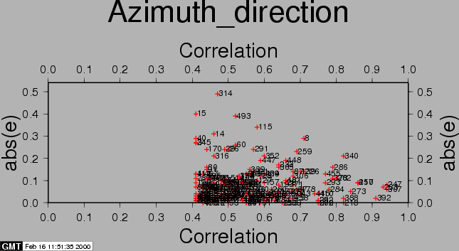
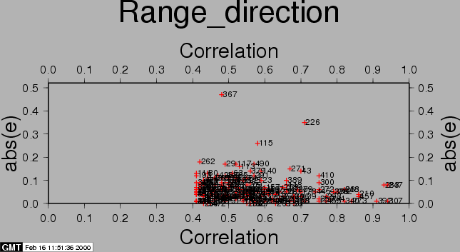
After the computations, the residuals between the estimated model and the 'observed' offsets are plotted with the csh-script plotcpm. These plots are useful to iteratively come to a good transformation model (changing CPM_THRESHOLD or CPM_DEGREE for each iteration, or identify and remove some estimated offsets (the 'observations', blunders) by setting their correlation to 0.00001 in the output section of the FINE processing step.

Also the observations itself and some statistics are plotted (w-tests, a large value indicates an unreliable estimate).

The script can be adapted to your own wishes, it simply calls GMT (see [19]) based on the ascii data file CPM_DATA.

This step is important, since the interferogram is sensestive to mis alignments of slave on master. Therefore, we always took a very cautious approach. However, that meant running this step, editing the result file, running again, etc. which got quite cumbersome. To reduce the manual effort, we introduced a card CPM_MAXITER that performs a number of iterations automatically. It also should remove no more windows than necessary for a good fit. I have experimented with values like 20 for this card. (having say 600 windows after step FINE). If you want to approach that after each computation you want to have full control what to do, simply set this card to 0.

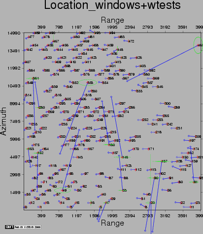
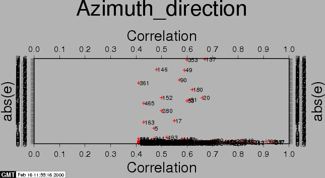
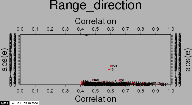
The first run of coregpm for the area of Fig. 23.1 is shown in Figures 20.1, 20.2, and 20.3. We have used a polynomial of degree 1, and a threshold of 0.4 here.

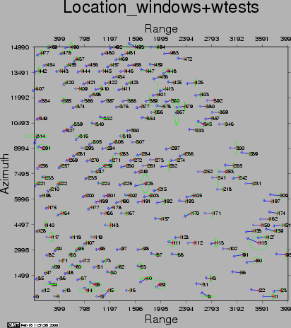
The second run of coregpm is shown in Figures 20.4, 20.5, and 20.6. In the products result file the outliers are artificially set to 0 correlation (thus being below the threshold), to exclude them from the least squares estimation. After this run we continued with the resampling.

**Figure 20.1:** Plot produced by 'plotcpm' for the first run. The estimated offsets are plotted here (normalized), together with a (90 degrees rotated) w test as ellipses.
$\begin{figure}\epsfig{file=Figures/coreg_errvector_wrong.eps,height=0.4\textheight}\end{figure}$

**Figure 20.2:** Plot produced by 'plotcpm' for the first run. The absolute error (estimated offsets minus observed offsets) are plotted for azimuth direction.
$\begin{figure}\epsfig{file=Figures/coreg_errazi_wrong.eps,height=0.3\textheight}\end{figure}$

**Figure 20.3:** Plot produced by 'plotcpm' for the first run. The absolute error (estimated offsets minus observed offsets) are plotted for the range direction.
$\begin{figure}\epsfig{file=Figures/coreg_errran_wrong.eps,height=0.3\textheight} \end{figure}$

**Figure 20.4:** Plot produced by 'plotcpm' for the second run. The estimated offsets are plotted here (normalized), together with a (90 degrees rotated) w test as ellipses.
$\begin{figure}\epsfig{file=Figures/coreg_errvector_ok.eps,height=0.4\textheight} \end{figure}$

**Figure 20.5:** Plot produced by 'plotcpm' for the second run. The absolute error (estimated offsets minus observed offsets) are plotted for azimuth direction.
$\begin{figure}\epsfig{file=Figures/coreg_errazi_ok.eps,height=0.3\textheight} \end{figure}$

**Figure 20.6:** Plot produced by 'plotcpm' for the second run. The absolute error (estimated offsets minus observed offsets) are plotted for the range direction.
$\begin{figure}\epsfig{file=Figures/coreg_errran_ok.eps,height=0.3\textheight} \end{figure}$

**Figure 20.7:** Plot produced by 'plotcpm'. The magnitude is plotted in the background.
$\begin{figure}\epsfig{file=Figures/plotcpm_bg.ps,height=0.4\textheight} \end{figure}$

Degree d=1 is enough to account for most effects in normal images. The 2d-polynomial has the form:

$\displaystyle f(x,y) = \sum_{i=0}^{d}\sum_{j=0}^{i} \alpha_{i-j, j} x^{i-j} y^{j}$

(T1)

Perhaps one might do the resampling with a lower quality polynomial, and thereafter do the fine coregistration (initial offsets 0,0) and this step (yielding new coefficients). The polynomial coefficient can then be added (?) to form a new model, with which the slave can again be resampled. This has not been tested.