Method: adaptive

After the resampling of the slave on the master grid is performed this algorithm can be used. The local fringe frequency is estimated using peak analysis of the power of the spectrum of the complex interferogram. The resampling is required since the local fringe frequency is estimated from the interferogram. This fringe frequency is directly related to the spectral shift in range direction. (Note this shift is not a shift, but different frequencies are mapped on places with this shift...) The algorithm generally works as follows.

• Take part of master and slave (e.g., 500 lines by 128 range pixels.)
• Oversample master and slave and generate complex interferogram.
• Take FFT over range for all lines of complex interferogram.
• Take power. If requested, weight this powerspectrum with auto-convolution of 2 rect functions with appropriate bandwidth. (Actually, perhaps the spectrum should also be weighted with autoconvolution of Hamming, but since I am not sure that this has a big impact on real data this is not done.)
• Take moving average over the lines of the power FFT's for noise suppression (kind of periodogram). (This was better implemented as a convolution with a block function (e.g., 9 x 128)?)
• Estimate peak per line in oversampled/averaged powerspectrum of complex interferogram. Estimate $SNR = {{{\rm fftlength} \cdot peak} \over {rest}}$.
• This peak is directly related to overlap of spectra for this part of this line. (See also Fig. 22.2.) $\Delta f_r = f_{\rm fringe}$.
• If SNR is above threshold (input of user, e.g., 3), remove appropriate parts of spectra of master/slave. Optionally compute inverse hamming window and new hamming window, and rect window to filter one side of master spectrum, and other side of slave spectrum. (See also Fig. 22.3.) Note that the filter is mirrored (matlab fliplr) for master/slave. The SNR of the peak of a random spectrum (sea) probably is a little larger than 1, so threshold of 3 may not be large enough.
• Do inverse FFT for filtered master, slave, which yields the filtered image in the space domain.
• Take next part of master and slave (e.g., 500 lines by next 128 range pixels) until all lines are filtered.

In practice this is done in blocks. These blocks are overlapping in lines (because the averaging over lines means one cannot filter all lines in the block), and not in range. Parameters that can be adjusted are the FFTlength, the moving average mean, the SNR threshold.

The fftlength should be large enough to yield a good estimate of the local fringe frequency, and small enough to contain a constant slope of the terrain. The total number of fringes in range directorion can be easily estimated using the perpendicular baseline.

It is probably a good idea to add a card so an overlap in range between blocks can be used. This avoids 'edge' effects, and increases the filtering of terrain near, e.g., a lake (since the SNR for peak detection will be higher for a number of blocks towards the noise). This is not implemented yet.

See also [5], [7], [3]. See also our matlab toolbox.

Figure 22.2: Peak estimation in spectral domain of (oversampled) complex interferogram. Non FFTshifted.

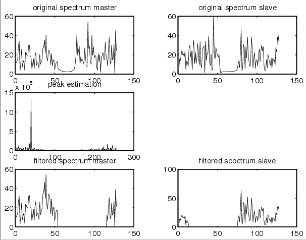Figure 22.3: Spectral filtering windows (inverse hamming, boxcar (rect), and new hamming. Note these are FFTshifted.

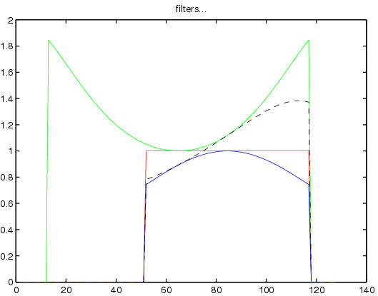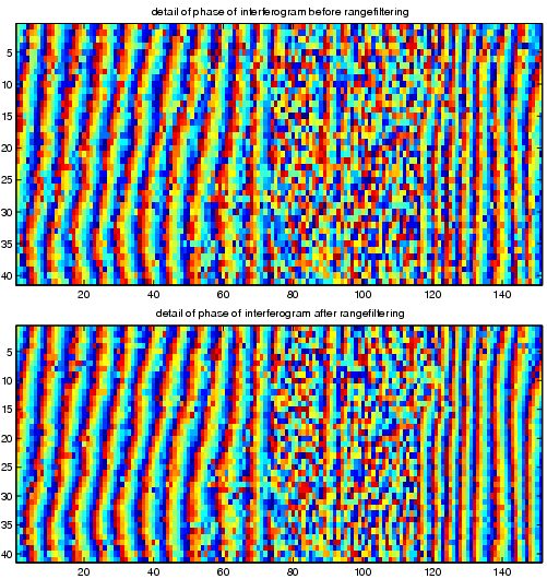
Figure 22.4: Detail of interferogram with and without rangefiltering. (fftlength=128, nlmean=15, snrtreshold=5). The perpendicular baseline is about 200 m for this interferogram. The fringes are clearly sharper after the filtering. The number of residues for the interferogram was reduced by 20%. Subtraction of both interferograms yielded a random phase, so no structural effect of range filter implemenation is suspected.