Using uniformly-distributed random generators ![]() , a one-dimensional
white circular Gaussian complex signal w is computed with
amplitude
, a one-dimensional
white circular Gaussian complex signal w is computed with
amplitude ![]() and phase
and phase ![]() . Low pass filtering yields a correlated
random signal. An oversampling ratio of 12.23 is used to create
the reference signal u, whereas the test signal
. Low pass filtering yields a correlated
random signal. An oversampling ratio of 12.23 is used to create
the reference signal u, whereas the test signal ![]() is a subsampled
version thereof. Using a subsampling ratio of
is a subsampled
version thereof. Using a subsampling ratio of ![]() reduces
the oversampling ratio of the test signal
to 1.223 to resemble ERS conditions.
The test signal
reduces
the oversampling ratio of the test signal
to 1.223 to resemble ERS conditions.
The test signal ![]() is then interpolated using the kernels under
investigation, yielding an estimate
is then interpolated using the kernels under
investigation, yielding an estimate ![]() of the reference signal.
The interpolation kernels nearest neighbor, piecewise
linear,
4-point and 6-point cubic convolution and
6-point, 8-point, and 16-point truncated sinc
are
created using the equations (6),(7),(8),
(9), and (10).
For every kernel the interferometric phase
error
of the reference signal.
The interpolation kernels nearest neighbor, piecewise
linear,
4-point and 6-point cubic convolution and
6-point, 8-point, and 16-point truncated sinc
are
created using the equations (6),(7),(8),
(9), and (10).
For every kernel the interferometric phase
error ![]() , the phase error
histogram, the total coherence
, the phase error
histogram, the total coherence ![]() and the standard deviation of
the interferometric phase error
and the standard deviation of
the interferometric phase error
![]() are evaluated.
Single experiment results of the interferometric phase error are shown
for the first 4 evaluated kernels in figure 4.
It can be seen that the variation of
the interpolated signal decreases considerably as the kernel contains
more sample points.
Nevertheless, spurious spikes up to
are evaluated.
Single experiment results of the interferometric phase error are shown
for the first 4 evaluated kernels in figure 4.
It can be seen that the variation of
the interpolated signal decreases considerably as the kernel contains
more sample points.
Nevertheless, spurious spikes up to ![]() still
cause residues in the interferogram.
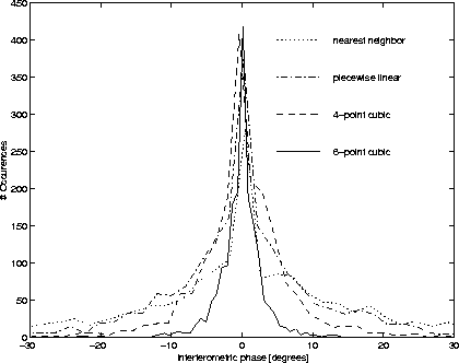
The histogram is depicted in figure 5.
The total coherence
still
cause residues in the interferogram.
The histogram is depicted in figure 5.
The total coherence ![]() and the standard deviation of the
interferometric phase
and the standard deviation of the
interferometric phase ![]() is studied using averaged values from 500
simulation loops. The results are given in table i, to allow
comparison with the theoretical findings. Coherence has been estimated
as the sample correlation coefficient of the reference signal u and
the interpolated signal
is studied using averaged values from 500
simulation loops. The results are given in table i, to allow
comparison with the theoretical findings. Coherence has been estimated
as the sample correlation coefficient of the reference signal u and
the interpolated signal ![]() .
.

Figure 5: Histogram of the phase errors for four kernels: nearest
neighbor, piecewise linear, 4-point cubic convolution, and
6-point cubic convolution.

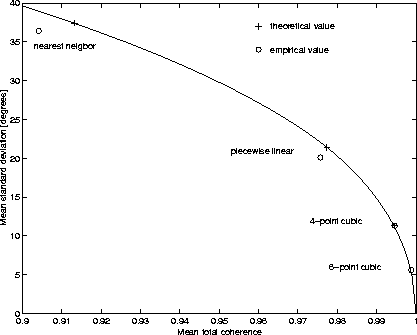
Figure 6: Phase standard deviation phase and coherence for
four interpolation kernels
Figure 6 shows the mean standard deviation of the phase as a function of the coherence for the four shortest kernels.