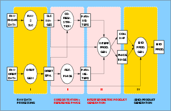
A high-level description of the InSAR processing is shown in Figure 1.1 where a division in four blocks has been made. Block I depicts the preprocessing of the raw (radar and orbit) data to another format.
We won't be concerned with the raw orbit data, but it is included in the flow chart for completeness. The Delft precise orbits are used for ERS1/2 and Envisat, obtained via the getorb package (see, e.g., [14]). The second block consists of the co-registration where the slave image is aligned with the master image, and of the computation of the reference phase of the ellipsoid. In block III the interferometric products (complex phase image and coherence map) are computed. Finally in block IV the endproducts (e.g., a DEM or a deformation map) are computed.
The processing steps that are implemented in the Doris software are listed in the table below. Note that UNWRAP is NOT directly implemented in Doris.
To run each step, these names must be used as arguments for the PROCESS card, as explained in Chapter 2. A specific algorithm (module, method) can be selected with the cards that are special to this step, see the Chapters 3 to 33.
| PROCESS (Chapter) | Description |
| M_READFILES (3) | Read the processing parameters from the SLC files for the master image. |
| M_PORBITS (4) | Retrieve the precise Delft orbital data records with the getorb package. |
| M_CROP (5) | Write the SLC data from paf format to disk in the 'raw' (pixel interleaved 2b/2b complex short integer) format. |
| M_SIMAMP (6) | Simulation of amplitude image based on DEM. |
| M_TIMING (7) | Estimation of timing error based on correlation between master amplitude and simulated amplitude. |
| M_OVS (8) | Oversampling of the master crop. |
| S_READFILES (9) | See M_READFILES. |
| S_PORBITS (10) | See M_PORBITS. |
| S_CROP (11) | See M_CROP. |
| S_OVS (12) | See M_OVS. |
| COARSEORB (13) | Compute the translation between master and slave with the orbits (precision 30 pixels). |
| COARSECORR (14) | Compute the translation between master and slave on pixel level by correlation technique. |
| M_FILTAZI (15) | Spectral filter for master image in azimuth (line) direction. |
| S_FILTAZI (16) | Spectral filter for slave image in azimuth (line) direction. |
| FINE (17) | Compute translation vectors over the total image on sub-pixel level. |
| RELTIMING (18) | Estimation of relative timing error between master and slave based on fine coregistration. |
| DEMASSIST (19) | DEM assisted coregistration. |
| COREGPM (20) | Compute the actual transformation (2d-polynomial) model for the alignment of the slave on the master image. |
| RESAMPLE (21) | Resample the slave image according to the transformation model of the coregistration. |
| FILTRANGE (22) | Spectral filter for master and slave image in range (pixel) direction. |
| INTERFERO (23) | Compute the (complex) interferogram. |
| COMPREFPHA (24) | Compute the reference phase of the ellipsoid to be subtracted from the interferogram (polynomial). |
| SUBTRREFPHA (25) | Subtract the reference phase of the ellipsoid from the interferogram. |
| COMPREFDEM (26) | Compute the reference phase of a DEM to be subtracted from the interferogram. |
| SUBTRREFDEM (27) | Subtract the reference phase of the DEM from the interferogram. |
| COHERENCE (28) | Compute the (complex) coherence map. |
| FILTPHASE (29) | Filter the the interferogram. |
| UNWRAP (30) | Unwrap the interferogram. |
| DINSAR (31) | 3/4 pass differential interferometry. |
| SLANT2H (32) | Compute the heights of the pixels in the radar coded system. |
| GEOCODE (33) | Geocode the pixels (convert pixels from the radar coordinate system to a earth fixed reference system.) |